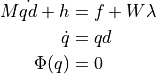
PyMbs translates the description based on bodies, joints and load elements
into the following system of differential equations describing the equations of
motion:
where is vector of the generalised positions; is the
vector of generalised velocities; is the vector of constraint
forces; is the generalised Mass Matrix; is a vector
containing all centrifugal and Coriolis forces; comprises all
internal and external loads; describes all holonomic
constraints.
Currently, PyMbs features an explicit and a recursive scheme to derive the
equations of motion. The explicit scheme is best used for small systems with up
to four degrees of freedom. It obtains expressions for , ,
, directly. This code is very compact for small systems
but the expressions become extremely long for larger systems. For that reason a
recursive scheme has been implemented which exploits the kinematic structure of
the system leading to many but simple equations.
The explicit scheme is based on the Newton-Euler-Algorithm and the symbolic
calculation capabilities of PyMbs through the use of sympy. Since an exhaustive
presentation would go far beyond the scope of this document, only the essential
highlights will be discussed.
Given a rigid body which is able to move freely in a three
dimensional space, following equations describe the trajectory of its centre of
gravity.
Where and describe the position and the velocity of
the centre of gravity with respect to the inertial frame;
represents its angular velocity with respect to a body-fixed frame;
describes the bodies orientation using Cardan Angles, for
example. and are sub matrices of the block
diagonal matrix , given by
with being the mass and being the symmetric tensor
of inertia. The vector contains centrifugal and
Coriolis-forces; comprises all internal and external forces and
torques.
Usually, a single body without any constraints will not be sufficient for a
model of a technical system. Multiple bodies, connected by joints or
governed by constraints are needed. Based on equation (2)
one can find a more general description for a system consisting of
bodies.
Although equation (3) looks very similar to equation
(2), the definitions of the used symbols does differ
, , , and are
generalised in a similar way.
Introducing joints between bodies leads to restrictions of their relative
movements for which algebraic constraints can be found
These constraints are ensured by introducing corresponding constraint forces
into the equations of motion acting perpendicular to the direction of allowed
displacements. Thus equation (3) changes to
Multiplication by from the left transforms the equation into
the space of the minimal coordinates, eliminating all influences of
constraint forces. This is due to the fact that no work is performed by
constraint forces since they always act perpendicular to the allowed
displacements. Thus equation (7) becomes
Since the explicit scheme is only suitable for small multibody systems an
explicit scheme has been implemented. This has been done according to [FS]
where a detailed explanation is given. Therefore only the implemented
equations will be given here.
For each body following information must be provided
Mass:
Inertia:
Position of Centre of Gravity:
Distance to all child bodies =
The underlying assumption is that every joint has exactly one degree of
freedom. More complex joints can be obtained through a combination of such
simple joints. In general each joint belonging to the body
has two parameters:
Axis of Translation:
Axis of Rotation:
The equations are generated in three steps. First there is a forward loop,
where all positions and velocities of each body is obtained. Below you find all
equations (taken from [FS]) with denoting the current body and
denoting its parent body. The index runs over all ancestor
bodies.
All values are initialised with except for
with denoting the gravity vector.
Second there is a backward loop in which all joint forces are calculated, with
denoting all direct successors (child bodies) of the body .
Third, there is another forward loop in which expressions for the generalised
accelerations are calculated.
The so found and are the elements of the Mass
Matrix and a -Vector which satisfies the following relation
A unique feature of PyMbs is its ability to deal with certain kinematic loops
in an explicit manner. This consequently leads to a formulation based on
minimal coordinates and thereby to explicit ordinary differential equations
without algebraic constraints. The underlying concept shall be presented in
this section.
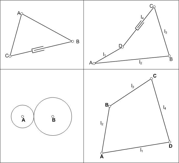
Currently, there are four different kinematic loops implemented as shown in
Figure Kinematic loops.
Left to right, top: CrankSlider, FourBarTrans. Bottom: Transmission,
FourBar
Handling kinematic loops is based on the coordinate partitioning method [WH].
Given the vectors of generalised positions , a set of independent
coordinates and a set of dependent coordinates are chosen
according to the definitions made in the kinematic loops.
First, an explicit relation between the dependent coordinates and
the independent coordinates must be provided for each loop.
Exploiting the (usually much simpler) implicit relation
of the loop , corresponding relations on velocity and acceleration
level may be derived.
with . The same can be achieved for finding a
relationship on acceleration level.
with . Thus, the equations the equations of motion can
be reduced even further, so that they only need to be solved for the set of
independent coordinates. Equation (1) may be rewritten using
equation (10).
Multiplying this equation with from the left yields
with ; ;
. Clearly, equation (11) has the form of
(1) and is therefore compatible.
In order to implement explicit handling for a new kinematic loop, the following
information must be provided:
partitioning of joint coordinates into and
, such that
, , such that
and
Note, that saving and directly, although they
can be derived from automatically, saves time when
assembling a model and leaves room for optimising these expressions towards
brevity.
Fisette, P; Samin, J. C.: Symbolic generation of large multibody system dynamic equations using a new semi-explicit Newton/Euler recursive scheme. In: Archive of applied mechanics Vol. 66, No 3. (1996) pp. 187-199
Wehage, R. A.; Hung, E. I.: Generalized coordinate partitioning for dimension reduction in analysis of constrained dynamic systems. I, Mech. Design 134 (1982) pp. 247-255
 is vector of the generalised positions;
  is the
vector of generalised velocities;
is the
vector of generalised velocities;  is the vector of constraint
forces;
is the vector of constraint
forces;  is the generalised Mass Matrix;
  is a vector
containing all centrifugal and Coriolis forces;
is a vector
containing all centrifugal and Coriolis forces;  comprises all
internal and external loads;
comprises all
internal and external loads;  describes all holonomic
constraints.
describes all holonomic
constraints. directly. This code is very compact for small systems
but the expressions become extremely long for larger systems. For that reason a
recursive scheme has been implemented which exploits the kinematic structure of
the system leading to many but simple equations.
directly. This code is very compact for small systems
but the expressions become extremely long for larger systems. For that reason a
recursive scheme has been implemented which exploits the kinematic structure of
the system leading to many but simple equations. which is able to move freely in a three
dimensional space, following equations describe the trajectory of its centre of
gravity.
which is able to move freely in a three
dimensional space, following equations describe the trajectory of its centre of
gravity.![\underbrace{
\left[\begin{array}{cc}
M_{1,i} & 0\\
0 & M_{2,i}\end{array}\right]}_{M_{i}}
\left[\begin{array}{c}
\dot{v}_{i}\\
\dot{\omega}_{i}\end{array}\right]+\underbrace{\left[\begin{array}{c}
0\\
\tilde{\omega}_{i}M_{2,i}\omega_{i}\end{array}\right]}_{h_{i}} &= \underbrace{\left[\begin{array}{c}
f_{e,i}\\
m_{e,i}\end{array}\right]}_{f_{i}}\\
v_{i} &= \dot{r}_{i}\\
\omega_{i} &=
H_{i}\dot{\alpha}_{i}](../_images/math/f4434b0216ddd69819e94b5d647d27695e9a74a0.png)
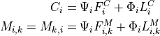
 and
and  describe the position and the velocity of
the centre of gravity with respect to the inertial frame;
describe the position and the velocity of
the centre of gravity with respect to the inertial frame;  represents its angular velocity with respect to a body-fixed frame;
 describes the bodies orientation using Cardan Angles, for
example.
describes the bodies orientation using Cardan Angles, for
example.  and
and  are sub matrices of the block
diagonal matrix
are sub matrices of the block
diagonal matrix  , given by
![M_{1,i} &= \left[\begin{array}{ccc} m_{i} & 0 & 0\\
0 & m_{i} & 0\\
0 & 0 & m_{i}\end{array}\right] \\
M_{2,i}=I_{i} &= \left[\begin{array}{ccc}
I_{xx,i} & I_{xy,i} & I_{xz,i}\\
I_{xy,i} & I_{yy,i} & I_{yz,i}\\
I_{xz,i} & I_{yz,i} & I_{zz,i}\end{array}\right]](../_images/math/7f87c6a38a1e473ba2a1fd76cabec1617d76054c.png)
 being the mass and
  being the symmetric tensor
of inertia. The vector
being the symmetric tensor
of inertia. The vector  contains centrifugal and
Coriolis-forces;
contains centrifugal and
Coriolis-forces;  comprises all internal and external forces and
torques.
comprises all internal and external forces and
torques. bodies.
![\underbrace{\left[\begin{array}{cc}
M_{1} & 0\\
0 & M_{2}
\end{array}\right]}_{M}
\left[\begin{array}{c}
\dot{zd}_{1}\\
\dot{zd}_{2}\end{array}\right]+\underbrace{\left[\begin{array}{c}
0\\
\tilde{zd}_{2}M_{2}zd_{2}\end{array}\right]}_{h} &=
\underbrace{\left[\begin{array}{c} f_{e}\\
m_{e}\end{array}\right]}_{f}\\
zd_{1} &= \dot{z}_{1}\\
zd_{2} &= H\dot{z}_{2}](../_images/math/047b97bcca1a0457f18c55254e88f007071e5d73.png)
![z_{1}=\left[\begin{array}{cccc}
r_{1}^{T} & r_{2}^{T} & \ldots & r_{N}^{T}\end{array}\right]^{T}
zd_{2}=\left[\begin{array}{cccc}
\omega_{1}^{T} & \omega_{2}^{T} & \ldots & \omega_{N}^{T}\end{array}\right]^{T}
M_{1}=blkdiag\left(M_{1,1},M_{1,2},\ldots,M_{1,N}\right)](../_images/math/d7cbca37c2733b2ff67224815d36d1e8c0b1cfbd.png)
 ,
,  ,
,  ,
,  and
and  are
generalised in a similar way.
are
generalised in a similar way.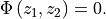
![M\left[\begin{array}{c}
\dot{zd}_{1}\\
\dot{zd}_{2}\end{array}\right]+h &= f+\left(\frac{\partial\Phi}{\partial
z}\right)^{T}\lambda\\
zd_{1} &= \dot{z_{1}}\\
zd_{2} &= H\dot{z_{2}}\\
\Phi &=
0](../_images/math/253d98c19e18dba81495c0604545b7e13c950e7f.png)
![z=\left[\begin{array}{cc}
z_{1}^{T} & z_{2}^{T}\end{array}\right]^{T}](../_images/math/42fa874cff6225f3da923b246ea89c0ae3ae1bcf.png)
 and
and  such that
 and
and 


 ,
,
 and its derivatives
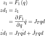
 ,
,  and its derivatives
 and
and  in equation
(4) by the newly found relations, gives
in equation
(4) by the newly found relations, gives![M\underbrace{\left[\begin{array}{c}
J_{T}\\
J_{R}\end{array}\right]}_{J}\dot{qd}+M\left[\begin{array}{c}
\dot{J}_{T}\\
\dot{J}_{R}\end{array}\right]qd+h=f+\left(\frac{\partial\Phi}{\partial
z}\right)^{T}\lambda](../_images/math/e47440fca649df5ef74664bbe7860af2acb81c59.png)
 from the left transforms the equation into
the space of the minimal coordinates, eliminating all influences of
constraint forces. This is due to the fact that no work is performed by
constraint forces since they always act perpendicular to the allowed
displacements. Thus equation (7) becomes
from the left transforms the equation into
the space of the minimal coordinates, eliminating all influences of
constraint forces. This is due to the fact that no work is performed by
constraint forces since they always act perpendicular to the allowed
displacements. Thus equation (7) becomes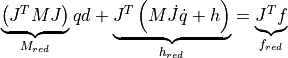


 runs over all ancestor
bodies.
runs over all ancestor
bodies.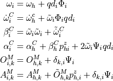
 except for
  with
with  denoting the gravity vector.
 denoting all direct successors (child bodies) of the body
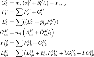
 and
and  are the elements of the Mass
Matrix
are the elements of the Mass
Matrix  -Vector which satisfies the following relation
 and a set of dependent coordinates
  are chosen
according to the definitions made in the kinematic loops.
are chosen
according to the definitions made in the kinematic loops.![q = \left[ \begin{array}{c}u\\v\end{array} \right]](../_images/math/fb3e07214ddc64e4ea0a8556c5371766aaaac46a.png)


 , corresponding relations on velocity and acceleration
level may be derived.
, corresponding relations on velocity and acceleration
level may be derived.
 . The same can be achieved for finding a
relationship on acceleration level.
. The same can be achieved for finding a
relationship on acceleration level.
 . Thus, the equations the equations of motion can
be reduced even further, so that they only need to be solved for the set of
independent coordinates. Equation (1) may be rewritten using
equation (10).
. Thus, the equations the equations of motion can
be reduced even further, so that they only need to be solved for the set of
independent coordinates. Equation (1) may be rewritten using
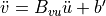
equation (10).![M\left(\underbrace{\left[\begin{array}{c}I\\
B_{vu}\end{array}\right]}_{J}\ddot{u}+\underbrace{\left[\begin{array}{c}
0\\
b^{\prime}\end{array}\right]}_{b}\right)+h &= F+W\lambda\\
MJ\ddot{u}+Mb+h &= F+W\lambda](../_images/math/92dd3b8ff5c5e102a026a51ce937398e140be5ae.png)
 ;
;  ;
;
 . Clearly, equation (11) has the form of
(1) and is therefore compatible.
. Clearly, equation (11) has the form of
(1) and is therefore compatible.
 ,
,  , such that
 and
and
 directly, although they
can be derived from
directly, although they
can be derived from  automatically, saves time when
assembling a model and leaves room for optimising these expressions towards
brevity.
automatically, saves time when
assembling a model and leaves room for optimising these expressions towards
brevity.