Getting Started
This section is meant to be a quick start guide and shall provide an overview of the basic features and capabilities of the PyMbs module. For a more detailed description please consult the Command Reference.
What is PyMbs?
PyMbs is a tool to generate the equations of motion of holonomic multibody systems. The equations can be exported to several target languages like Matlab, Modelica, Python or C++. Thus the output of PyMbs is a mathematical model of the mechanical system which can be simulated by timestep integration [1].
The description of the mechanical system is text-based but held as easy and convenient as possible. The user assembles the system from a range of predefined objects like bodies, joints, loops and sensors. As this method may provoke typing errors, especially when modelling more complex systems, it is possible to create a visualisation for the mechanical system from CAD files or geometric primitives to check the consistency of the model. It is also possible to manipulate the degrees of freedom interactively.
Installation
Warning
This installation guide is outdated. Basically you have to
clone the repo from GitHub
use CMake to build the C++ symbolics module
add pymbs to your environment/path so that it can be imported
We hope to have a package available again for convenience. Any help is highly appreciated…
PyMbs has been tested and works on Windows 10, Fedora Linux and Apple M1.
Note
A C-compiler must be available in the PATH to compile the model in the GUI for faster simulation. GCC is recommended as it works out of the box on Windows and Linux.
Warning
There is an issue under Wayland on Linux preventing the PyMbs window from being shown. To workaround the issue do
export QT_QPA_PLATFORM=xcb
in your shell / session (see https://github.com/pyvista/pyvistaqt/issues/445)
Outdated! It was tested on Python 2.7. In this section the required modules are specified and afterwards a step-by-step instruction is given on how to install PyMbs on Windows machines, which is intended to help users who never got in touch with Python before.
Dependencies
See requirements.txt in the project root folder for all dependencides. The most important are
numpy
scipy
vtk
matplotlib
PySide6
Windows
This guide assumes that no Python distribution is installed on your system. If Python is already installed, you may go directly to A First Example. We strongly recommend the installation of a prebundled Python distribution to avoid troubles regarding dependencies.
Download Python(x,y) from http://www.pythonxy.com.
Install Python(x,y). Make sure you selected ‘Full’ as ‘type of install’. This will install Python 2.7 to ‘C:\Python27’ and Python(x,y) to ‘C:\Program Files\pythonxy’ per default.
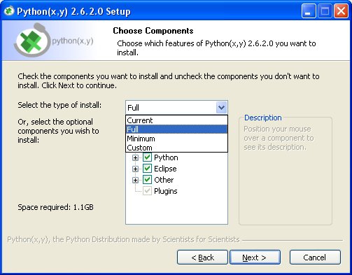
Python(x,y) installer
Install PyMbs using the installer PyMbs-0.2.1-alpha.win32.exe.
Note that this programme must be run with administrator privileges. Please make sure that PyMbs uses the correct Python Version which is in ‘C:\Python27’ per default. This is especially important if there is more than one Python distribution installed.
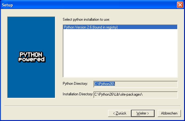
PyMbs installer
You may use any text editor to write your PyMbs models. However, we recommend the use of PyScripter as it supports syntax highlighting and code completion. It is freely available at http://code.google.com/p/pyscripter/.
You can check your installation by starting Python(x,y) from your desktop and pressing the button next to IPython(x,y) which will start IPython. As soon as IPython has started a line saying
In [1]:will appear. Now typefrom PyMbs.Input import *. If there is no error message and it jumps directly toIn [2]:then the installation was successful.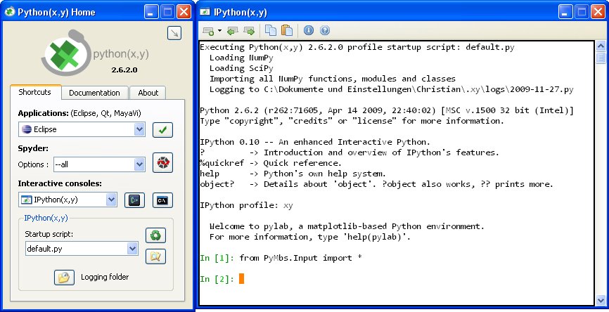
Check your installation
Linux
Currently, there are no PyMbs binaries for Linux. However, you can build PyMbs yourself. All you need is a C++ Compiler, CMake and various python packages, specifically numpy, scipy, matplotlib, vtk and PyQt4. Under Debian and Ubuntu, you can install these with:
sudo apt-get install build-essential cmake python-numpy python-scipy python-vtk python-qt4 python-h5py python-matplotlib
Then all you have to do to build and install PyMbs is:
sudo python setup.py install
Mac OS
As we don’t have a Mac available for testing, we can’t give any instructions for installing. Basically, if you have Python and its modules running, you only need to copy the PyMbs package to a folder of your choice and add it to the PYTHONPATH.
A First Example
Mechanical System
In order to demonstrate the usage of PyMbs a simple exemplary system shall be modeled. Consider the system of a crane crab given in figure PyMbs visualisation of the crane crab.
Model Description
Next the model of the crane crab is generated using PyMbs.
Start PyScripter (or your favourite Python editor) and copy the following code into the editor window. Please note that some systems mess up the apostrophe ‘?! If that is the case it is marked as red and has to be replaced manually by a proper one.:
# import PyMbs
from pymbs.input import *

# set up inertial frame
world=MbsSystem([0,0,-1])

# add inputs and parameters
F=world.addInput('F', limits=[-10, 10], name='DrivingForce')
m1=world.addParam('m1', 1.0)
m2=world.addParam('m2', 1.0)
l2=world.addParam('l2', 1.0)
I2=world.addParam('I2', (m2*l2**2)/12)

# add bodies
crab=world.addBody(mass=m1, name='Crab')
pend=world.addBody(mass=m2, inertia=diag([0,I2,0]), name='Pendulum')
pend.addFrame(name='joint' , p=[0, 0, l2])
pend.addFrame(name='middle', p=[0, 0, l2/2], R=rotMat(pi/2,'x'))

# add joints
jT = world.addJoint(world, crab, 'Tx', 1, name='TransCrab')
jR = world.addJoint(crab, pend.joint, 'Ry', -1, name='RotPendulum')

# add load element and sensor
world.addLoad.CmpForce([F,0,0], crab, world)
world.addSensor.Distance('d', crab, world)

# add visualisation
world.addVisualisation.Box(crab, 1, 0.5, 0.1)
world.addVisualisation.Cylinder(pend.middle, 0.01, 1)
world.addVisualisation.Sphere(pend, 0.1)

# generate equations
world.genEquations.Explicit()

# generate simulation code
world.genCode.Python('CraneCrab', './Output')

# show system
world.show('CraneCrab')
Once you have done this, you can run the model by clicking on the button with a green arrow inside. After a short moment you should see a screen showing the crane crab (figure PyMbs visualisation of the crane crab). You may use the sliders on the left to move the crane crab and the pendulum which can be used for checking the kinematics of your assembly. In case you receive a Syntax Error you might have to replace the inverted commas by ‘proper ones’. Also note that, due to the fact that PyScripter does not properly reinitialise its Python engine, it might help to restart it as soon as you receive errors you cannot explain.
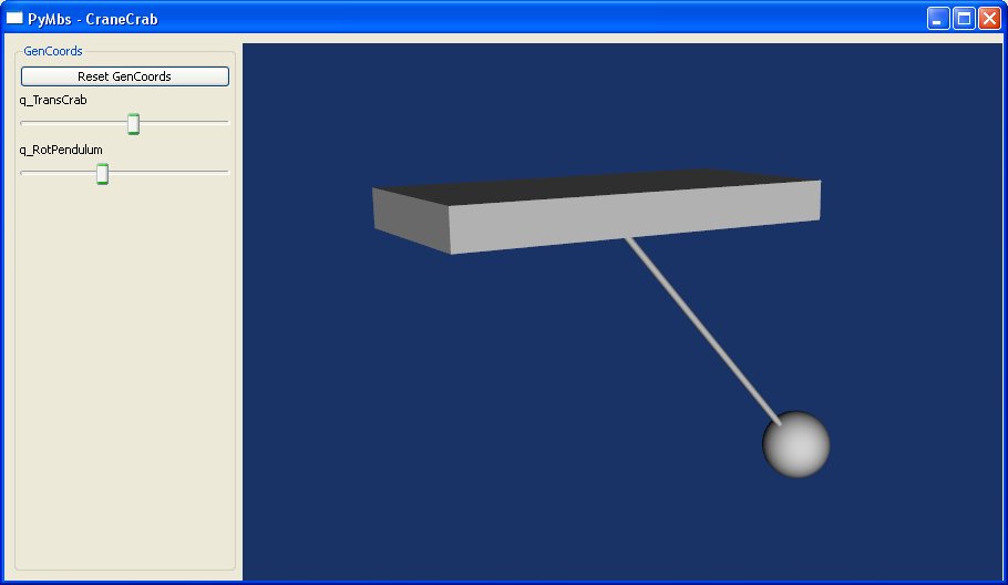
PyMbs visualisation of the crane crab
Code Export
Python
The command world.genCode('py', 'CraneCrab') is used to export the
equations of motion into Python format. The generated module
CraneCrab_der_state.py includes the function CraneCrab_der_state(t,
y) which calculates the state derivative from a given state. This can be used in combination with any standard numerical integrator, which is able to solve differential equations of the form

where y is the state vector and t the time.
Modelica
The Modelica code generator, accessible through world.genCode('mo','CraneCrab'), creates a file called
CraneCrab_der_state.mo. It can be used in combination with any Standard
Modelica tool such as OpenModelica (http://www.openmodelica.org) or
JModelica (http://www.jmodelica.org). Note, that this special model is defined partial since no equation for the input F is given. Usually, the driving force F is calculated directly inside Modelica using the Modelica Standard Library (MSL). In order to combine this model with the MSL, it is recommended to write another Modelica model by hand as given in the listing below which inherits from the automatically generated
model and simply extends it by a mechanical connector:
model CraneCrab
extends CraneCrab_der_state;
        import Modelica.Mechanics.Translational.*;
        Interfaces.Flange_b flange;
equation
        flange.f = F;
        flange.s = d[1];
end CraneCrab;
Matlab
The MATLAB code generation is more involved since five different files are generated
CraneCrab_sim.m Basic simulation file. It defines the initial values, start time and stop time and calls the solver.
CraneCrab_der_state.m This file features the calculation of all state derivatives of the form

CraneCrab_inputs.m This function is called from CraneCrab_der_state.m. Here one can implement its own algorithms to generate inputs to the system.
CraneCrab_sensors.m PyMbs separates the calculation of sensor values from the state derivatives. The function within CraneCrab_sensors returns a struct containing all sensor values if passed a state vector, i.e.

CraneCrab_visual.m This file can be used to visualise the system according to the description in the PyMbs model description. It features a function that takes the result from the MATLAB Solvers, i.e. a vector T containing all time values and a matrix Y where each row is a state vector. The column corresponds to the time value in T. There is third parameter fak which can be used to slow the visualisation down if chosen greater than one.
Footnotes