Inverted Pendulum

In this example, we would like to introduce the controller functionality of PyMbs. With it, you can introduce loads depending on the state of the system using arbitrary python code. We want to simulate a simple pendulum hanging from a travelling trolley, with a force acting on the trolley to keeep the pendulum in an upright position. If you want to try it first, or look at the complete source code, see inverted_pendulum.py. Note: You’ll also need the corresponding controller.py to run the example.

We will start again with importing PyMbs, but also importing the controlForce residing in our controller.py. We also set up our initial frame of reference:

import os

from pymbs.input import MbsSystem
from controller import controlForce

# path to 3D-models
models = os.path.join(os.path.dirname(__file__), '../../stl')

world = MbsSystem([0, 0, -1])

We add the masses of the trolley and the load, as well as the two bodies themselves:

M1 = world.addParam('m1', 0.8)
M2 = world.addParam('m2', 0.3)

Trolley = world.addBody(M1)
Load = world.addBody(M2, cg=[0, 0, -0.5])

The trolley can move translational and the pendulum rotates around the mounting point at the trolley. Note that we need to set the inital values here. The controller is rather basic and only works in a limited start angle range of the pendulum:

world.addJoint(world, Trolley, 'Tx', startVals=0.6)
world.addJoint(Trolley, Load, 'Ry', startVals=2.3)

Now the interesting bit. First, we add a controller, which gets a symbol 'F', the handle of the function describing the controller controlForce and for non-scalar controllers, the resulting shape (3, ), i.e. this controller returns a vector:

F = world.addController('F', controlForce, shape=(3, ))

Now we can use this object in any expression or load we would like. Here we add a CmpForce between the world and the trolley:

world.addLoad.CmpForce(F, Trolley, world, name='DrivingForce')

Let’s take a quick look at the controller itself. The source code is

import numpy as np

def controlForce(t, y, sensors):
    k = [ 25.4841998, 83.5330999,  20.38735984, 18.19367992]
    y0 = np.r_[0, np.pi, 0 ,0]
    F = np.dot(y-y0, k)
    return np.r_[F, 0, 0]

If you want to supply your own controller, the function has to adhere to the format functionname(time, coordinatevec, sensors), where time is the current simulation time, coordinatevec is a vector containing the generalised coordinates and their time derivative. In this example, we take the difference between the current generalised coordinates y and the point we would like to reach y0 and multiply this by the vector k, which was predetermined for the particular parameters of this example. Of course, you could just as well calculate it in this function. The result is the x-component of our force.

All that is left is to define the visualisations, generate our equations of motion and take a look at the system:

# Visualisation
world.addVisualisation.Box(world, length=3, width=0.05, height=0.05)
world.addVisualisation.Box(Trolley, length=0.1, width=0.1, height=0.1)
world.addVisualisation.File(Load, os.path.join(models, 'load.stl'))

# Generate equations and show model
world.genEquations.Recursive()
world.show('InvertedPendulum')

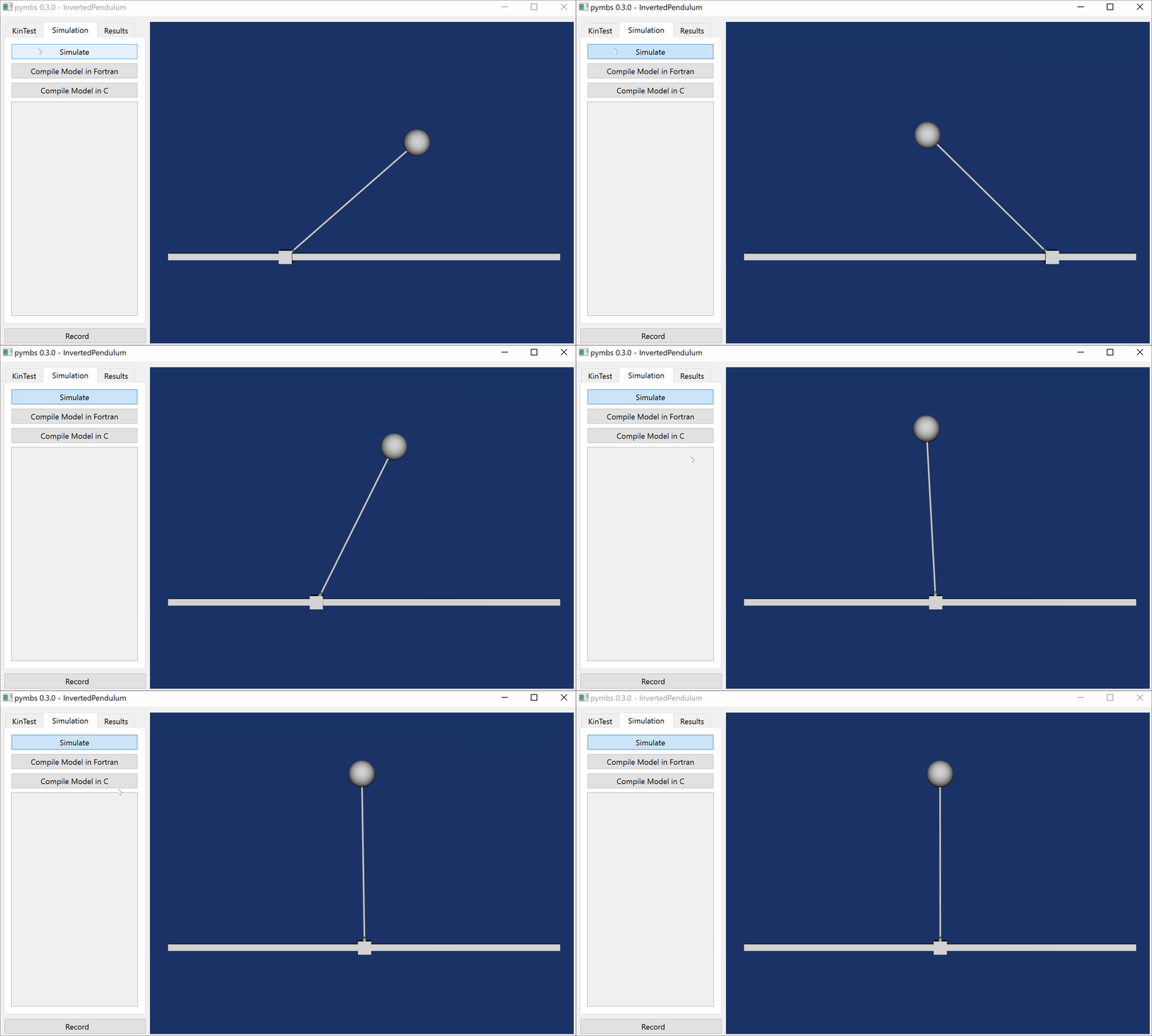
This results from running the simulation:

In the end, the complete source looks like this:

"""
Controlled pendulum

Single pendulum with controlling force acting on the joint. The control force
is defined in `controller.py` and tries to keep the pendulum upright.
If you set the initial angle to 2.4 or more, the controller should reach
equilibrium.
"""

# Warning: The source code of the examples is quoted in the documentation. If
# you change this file, you'll have to change the corresponding file in the
# documentation (see doc/examples).

import os

from pymbs.input import MbsSystem
from controller import controlForce

# path to 3D-models
models = os.path.join(os.path.dirname(__file__), '../../stl')

world = MbsSystem([0, 0, -1])

M1 = world.addParam('m1', 0.8)
M2 = world.addParam('m2', 0.3)

Trolley = world.addBody(M1)
Load = world.addBody(M2, cg=[0, 0, -0.5])

world.addJoint(world, Trolley, 'Tx', startVals=0.6)
world.addJoint(Trolley, Load, 'Ry', startVals=2.3)

F = world.addController('F', controlForce, shape=(3, ))
world.addLoad.CmpForce(F, Trolley, world, name='DrivingForce')

# Visualisation
world.addVisualisation.Box(world, length=3, width=0.05, height=0.05)
world.addVisualisation.Box(Trolley, length=0.1, width=0.1, height=0.1)
world.addVisualisation.File(Load, os.path.join(models, 'load.stl'))

# Generate equations and show model
world.genEquations.Recursive()
world.show('InvertedPendulum')