Mass-Spring-Damper System

Another commonly used introductory system is the mass-spring-damper system. A mass connected to a spring and a damper is displaced and then oscillates in the absence of other forces. If you want to try it first, or look at the complete source code, see mass_spring_damper.py.

As in the previous example, we import PyMbs, set up an intial reference frame and add a few parameters:

from pymbs.input import MbsSystem

world = MbsSystem([0, 0, -1])
m = world.addParam('m', 1)
c = world.addParam('c', 10)
d = world.addParam('d', 0.2)

Now we add the mass to the system and add a joint. Tz means that the mass can only undergo translation in z-direction. None of this is really new, but we add another parameter to the joint, startVals=1, which means the mass will have an initial displacement of one:

movingBody = world.addBody(m)
world.addJoint(world, movingBody, 'Tz', startVals=1)

This is where it gets interesting. We want to add a force to the system to simulate the influence of a spring and damper on the mass. First, we need to know the displacement and velocity of the mass. Therefore, we add a distance sensor:

l = world.addSensor.Distance('l', movingBody, world)

The Distance sensor measures the scalar distance between two coordinate systems, here the systems of movingBody and world. Additionally, it measures the velocity. You can access the distance with l[0] and the velocity with l[1]. The force for a spring is $F_s = - c x$ , with $c$ being the spring constant, and for a damper with a damping coefficient of $d$ the force is $F_d = - d \dot{x}$ . Therefore, we add an expression that includes both:

F = world.addExpression('F', -(c * l[0] + d * l[1]))

So far, this only calculates the value of the force, but it isn’t applied to the system. To change this, we add a PtPForce between the body and the world:

world.addLoad.PtPForce(F, movingBody, world)

As in the previous example, we need to add visualisations so that we can see the movement of our system:

world.addVisualisation.Box(movingBody, 1, 1, 1)
world.addVisualisation.Frame(world)

In the end, we generate the equations of motion for our system and show the visualisation:

world.genEquations.Recursive()
world.show('MassSpringDamper')

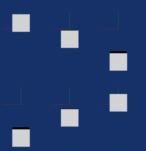
This is what it should look like:

In the end, the complete source looks like this:

"""
Model for a 1D mass attached to a parallel spring-damper.
"""

# Warning: The source code of the examples is quoted in the documentation. If
# you change this file, you'll have to change the corresponding file in the
# documentation (see doc/examples).

# set up PyMbs and the multi-body system
from pymbs.input import MbsSystem

world = MbsSystem([0, 0, -1])

# Add parameters
m = world.addParam('m', 1)
c = world.addParam('c', 10)
d = world.addParam('d', 0.2)

# Add the body and constrain its movement
movingBody = world.addBody(m)
world.addJoint(world, movingBody, 'Tz', startVals=1)

# Add force to simulate a spring-damper combination
l = world.addSensor.Distance('l', movingBody, world)
F = world.addExpression('F', -(c * l[0] + d * l[1]))
world.addLoad.PtPForce(F, movingBody, world)

# Add visualisations
world.addVisualisation.Box(movingBody, 1, 1, 1)
world.addVisualisation.Frame(world)

# Generate equations and show the system
world.genEquations.Recursive()
world.show('MassSpringDamper')